PLS-DA performance

2025-08-01

Introduction

This page presents an application of the PLSDA performance assessment. The PLS method is a quite particular method : there are several predictions according to the number of components selected in the model. It is the same with PLSDA. The goal is almost to choose the best number of components in PLS regression in order to compute the best possible predictions. For that, we will use two datasets:

• one is a dataset with only ten predictor variables $X = (X1,X2,...,X10)$ and two classes.

• the other is a dataset with forty predictor variables $X = (X1,X2,...,X40)$ and three classes. With $p = 40 > n = 30$, this dataset approches realist conditions for PLS training.

To access to predefined functions from sgPLSdevelop package and manipulate these datasets, run these lines :

library(sgPLSdevelop)
library(mixOmics)

data1 <- data.cl.create(p = 10) # 2 classes by default
data2 <- data.cl.create(n = 30, p = 40, classes = 3)

ncomp.max <- 8

# First model
X <- data1$X
Y <- data1$Y.f
model1 <- PLSda(X,Y, ncomp = ncomp.max)
model1.mix <- mixOmics::plsda(X,Y,ncomp = ncomp.max)

# Second model
X <- data2$X
Y <- data2$Y.f
model2 <- PLSda(X,Y, ncomp = ncomp.max)
model2.mix <- mixOmics::plsda(X,Y,ncomp = ncomp.max)

In the continuation of this article, we will show PLS-DA performance assessment with mean error rate by using leave-one-out cross-validation (LOOCV), 10-fold CV and 5-fold CV. The perf.PLSda function will allow to compute the error rate for each application case.

NB : there are three possible distances for computing the error rate : $\textit{maximum}$ distance, $\textit{centroïds}$ distance and $\textit{Mahalanobis}$ distance. By default, this function uses $\textit{maximum}$ distance. In the most complicated cases, it is advisable to choose $\textit{Mahalanobis}$ distance which gives more accurate results.

Leave-one-out CV

The Leave-one-out CV (LOOCV) builts $n$ models with a test set composed of only a single row (never the same row for each model).

First model

Let’s start with the first model.

perf.res1 <- perf.PLSda(model1, validation = "loo", progressBar = FALSE)

Error rate of the first model by LOOCV

h.best <- perf.res1$h.best

The perf.PLSda function gives us a optimal number of components equal to $H =$ 1, therefore we suggest to select 1 component(s) in our first model.

err <- round(perf.res1$error.rate,3)
#perf <- perf(model1.mix, validation = "loo", dist = "max.dist")
#err2 <- round(perf$error.rate$overall[1],3)
#data.frame(err,err2)

Second model

Let’s continue with the second model.

perf.res2 <- perf.PLSda(model2, validation = "loo", progressBar = FALSE)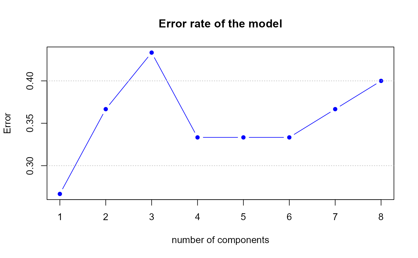

Error rate of the second model by LOOCV

h.best <- perf.res2$h.best

The perf.PLSda function gives us a optimal number of components equal to $H =$ 1, therefore we suggest to select 1 component(s) in our first model.

The LOOCV is an efficient way to assess performance but requires a large computing capacity. The K-fold CV (which create K blocks) reduces not only the number of models to built but also the execution time.

err <- round(perf.res2$error.rate,3)
perf <- perf(model2.mix, validation = "loo", dist = "max.dist")
err2 <- round(perf$error.rate$overall[1],3)
data.frame(err,err2)

##     err  err2
## 1 0.267 0.267
## 2 0.367 0.267
## 3 0.433 0.267
## 4 0.333 0.267
## 5 0.333 0.267
## 6 0.333 0.267
## 7 0.367 0.267
## 8 0.400 0.267

10-fold CV

The 10-fold CV builts 10 models. In our case, for each model, the test set is composed of 4 observations for the first model and 3 for the second.

First model

perf.res1 <- perf.PLSda(model1, folds = 10, progressBar = FALSE)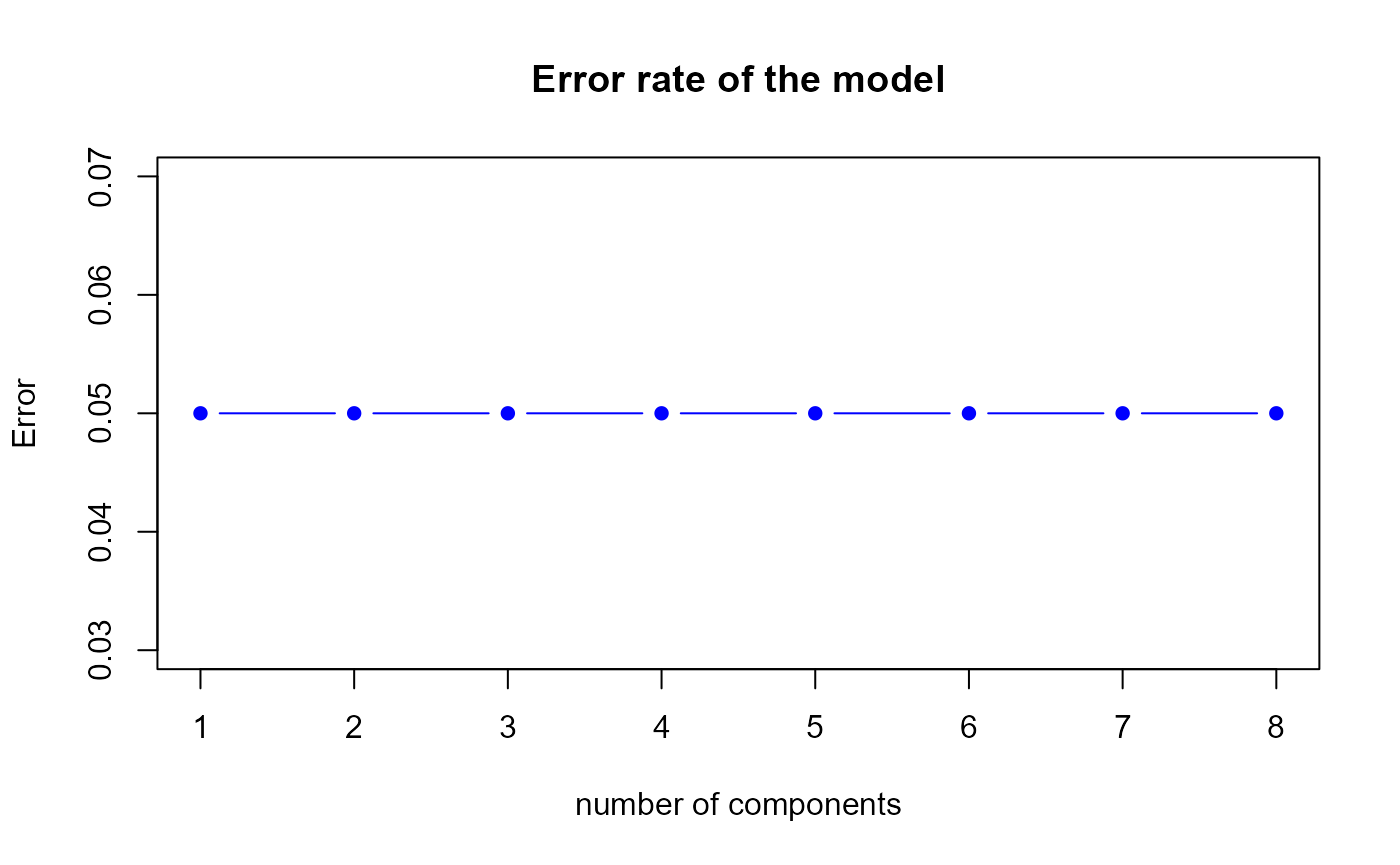

Error rate of the first model by 10-fold CV

h.best <- perf.res1$h.best

The perf.PLSda function gives us a optimal number of components equal to $H =$ 1.

err <- round(perf.res1$error.rate,3)
#perf <- perf(model1.mix, validation = "Mfold", folds = 10, dist = "max.dist")
#err2 <- round(perf$error.rate$overall[1],3)
#data.frame(err,err2)

Second model

perf.res2 <- perf.PLSda(model2, folds = 10, progressBar = FALSE)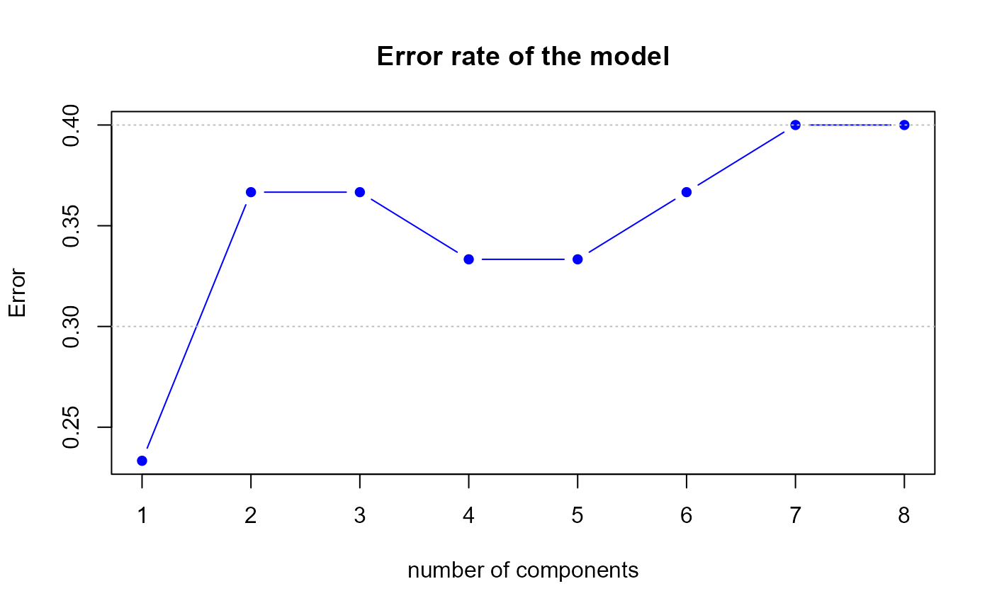

Error rate of the second model by 10-fold CV

h.best <- perf.res2$h.best

The perf.PLSda function gives us a optimal number of components equal to $H =$ 1.

err <- round(perf.res2$error.rate,3)
perf <- perf(model2.mix, validation = "Mfold", folds = 10, dist = "max.dist")
err2 <- round(perf$error.rate$overall[1],3)
data.frame(err,err2)

##     err  err2
## 1 0.233 0.133
## 2 0.367 0.133
## 3 0.367 0.133
## 4 0.333 0.133
## 5 0.333 0.133
## 6 0.367 0.133
## 7 0.400 0.133
## 8 0.400 0.133

5-fold CV

The 5-fold CV builts 5 models. In our case, for each model, the test set is composed of 8 observations for the first model and 6 for the second.

First model

perf.res1 <- perf.PLSda(model1, folds = 5, progressBar = FALSE)

Error rate of the first model by 5-fold CV

h.best <- perf.res1$h.best

The perf.PLSda function gives us a optimal number of components equal to $H =$ 1.

err <- round(perf.res1$error.rate,3)
#perf <- perf(model1.mix, validation = "Mfold", folds = 5, dist = "max.dist")
#err2 <- round(perf$error.rate$overall[1],3)
#data.frame(err,err2)

Second model

perf.res2 <- perf.PLSda(model1, folds = 5, progressBar = FALSE)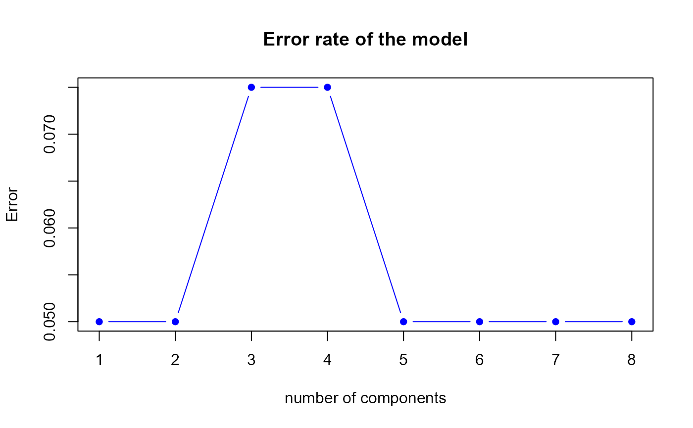

Error rate of the second model by 5-fold CV

h.best <- perf.res2$h.best

The perf.PLSda function gives us a optimal number of components equal to $H =$ 1.

err <- round(perf.res2$error.rate,3)
perf <- perf(model2.mix, validation = "Mfold", folds = 5, dist = "max.dist")
err2 <- round(perf$error.rate$overall[1],3)
data.frame(err,err2)

##     err  err2
## 1 0.050 0.133
## 2 0.050 0.133
## 3 0.075 0.133
## 4 0.075 0.133
## 5 0.050 0.133
## 6 0.050 0.133
## 7 0.050 0.133
## 8 0.050 0.133