sPLS performance

2025-07-30

Introduction

This page presents an application of the sPLS performance assessment. The sPLS method is a quite particular method : there are several predictions according to the components number selected in the model. The goal is almost to choose the best number of component in sPLS regression in order to compute the best possible predictions but also to select the best number of variables. For that, we will use three datasets:

• one is a dataset with only one response variable $Y$.

• the other is a dataset with four response variables $Y = (Y1,Y2,Y3,Y4)$.

• the last dataset contains real data about NIR spectra.

To access to predefined functions from sgPLSdevelop package and manipulate these datasets, run these lines :

library(sgPLSdevelop)
library(pls)

data1 <- data.create(p = 10, list = TRUE)
data2 <- data.create(p = 10, q = 4, list = TRUE)
data(yarn)
data3 <- yarn

## [1] "First dataset dimensions : 40 x 11"

## [1] "Second dataset dimensions : 40 x 14"

## [1] "Yarn dataset dimensions : 28 x 3"

For the two first datasets, the population is set to $n = 40$ by default, which is close to actual conditions. Let’s also notice that, on average, the response $Y$ is a linear combination from the predictors $X$. Indeed, the function includes a matrix product $Y = XB + E$ with $B$ the weight matrix and $E$ matrix the gaussian noise. This linearity condition is important in order to have a good performance of the model, the PLS method using linearity combinaison.

Now, it’s time to train a PLS model for each dataset built or imported.

ncomp.max <- 8

# First model
X <- data1$X
Y <- data1$Y
model1 <- sPLS(X,Y,mode = "regression", ncomp = ncomp.max)

# Second model
X <- data2$X
Y <- data2$Y
model2 <- sPLS(X,Y,mode = "regression", ncomp = ncomp.max)

# Third model
X <- data3$NIR
Y <- data3$density
model3 <- sPLS(X,Y,mode = "regression", ncomp = ncomp.max)

sPLS performance assessment using MSEP

An good way to assess such a model performance consists by using $MSEP$ criterion. $MSEP$ is computed as follow :

$MSEP = \frac{1}{nq} \sum_{i=1}^{n} \sum_{j=1}^{q} (Y_{i,j} - \hat{Y}_{i,j})^2$

The function named perf.sPLS will allow to assess the performance and to choose the best parameters. This function outputs the best tuning parameters but also two MSEP plots : the one shows the MSEP according to the number of components and the other shows the MSEP according to the number of selected variables in $X$ and $Y$. Particularly, in multivariate sPLS ($q>1$), the “plot” is a table of MSEP values.

First model MSEP

perf.res1 <- tuning.sPLS.XY(model1)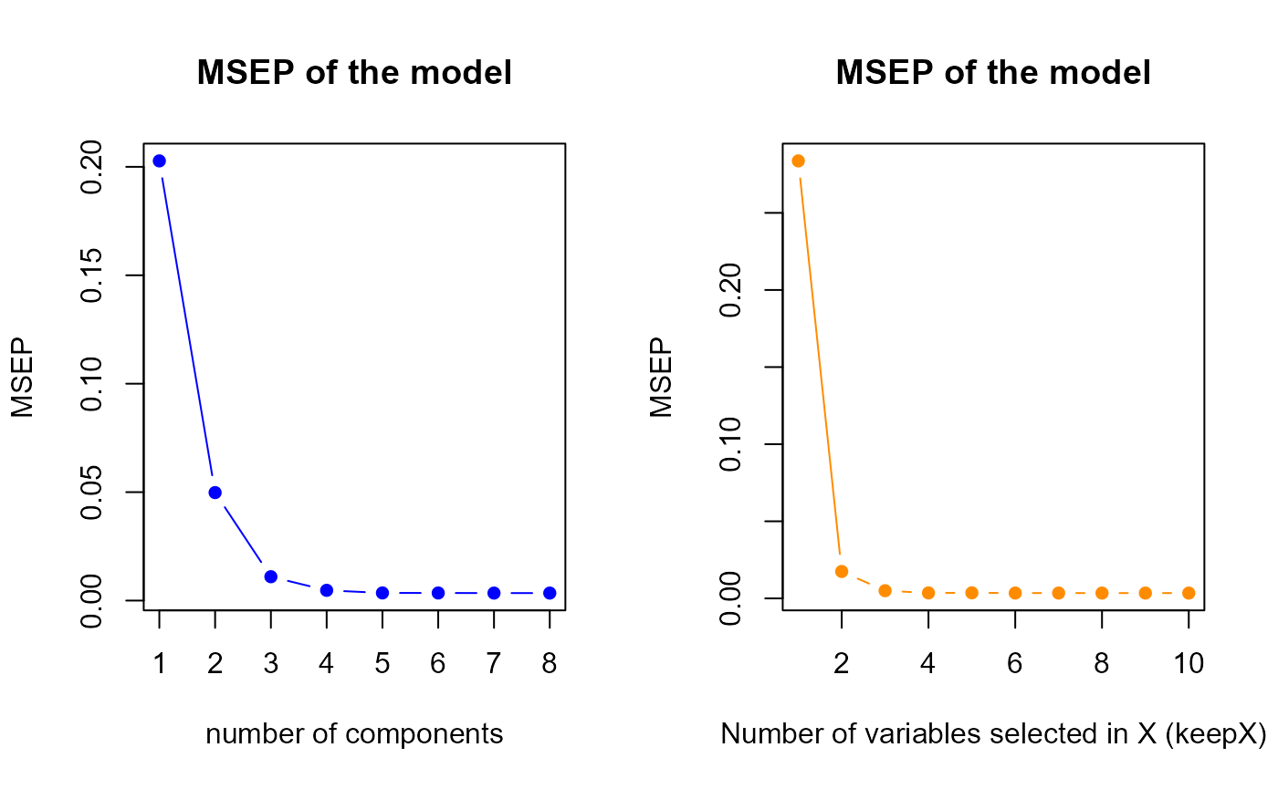

h.best <- perf.res1$h.best
keepX.best <- perf.res1$keepX.best
keepY.best <- perf.res1$keepY.best

The perf.sPLS gives us a optimal components number equal to $H =$ 7, therefore we suggest to select 7 components in our first model. It indicates us also to select 8 variables for each component.

Second model MSEP

perf.res2 <- tuning.sPLS.XY(model2)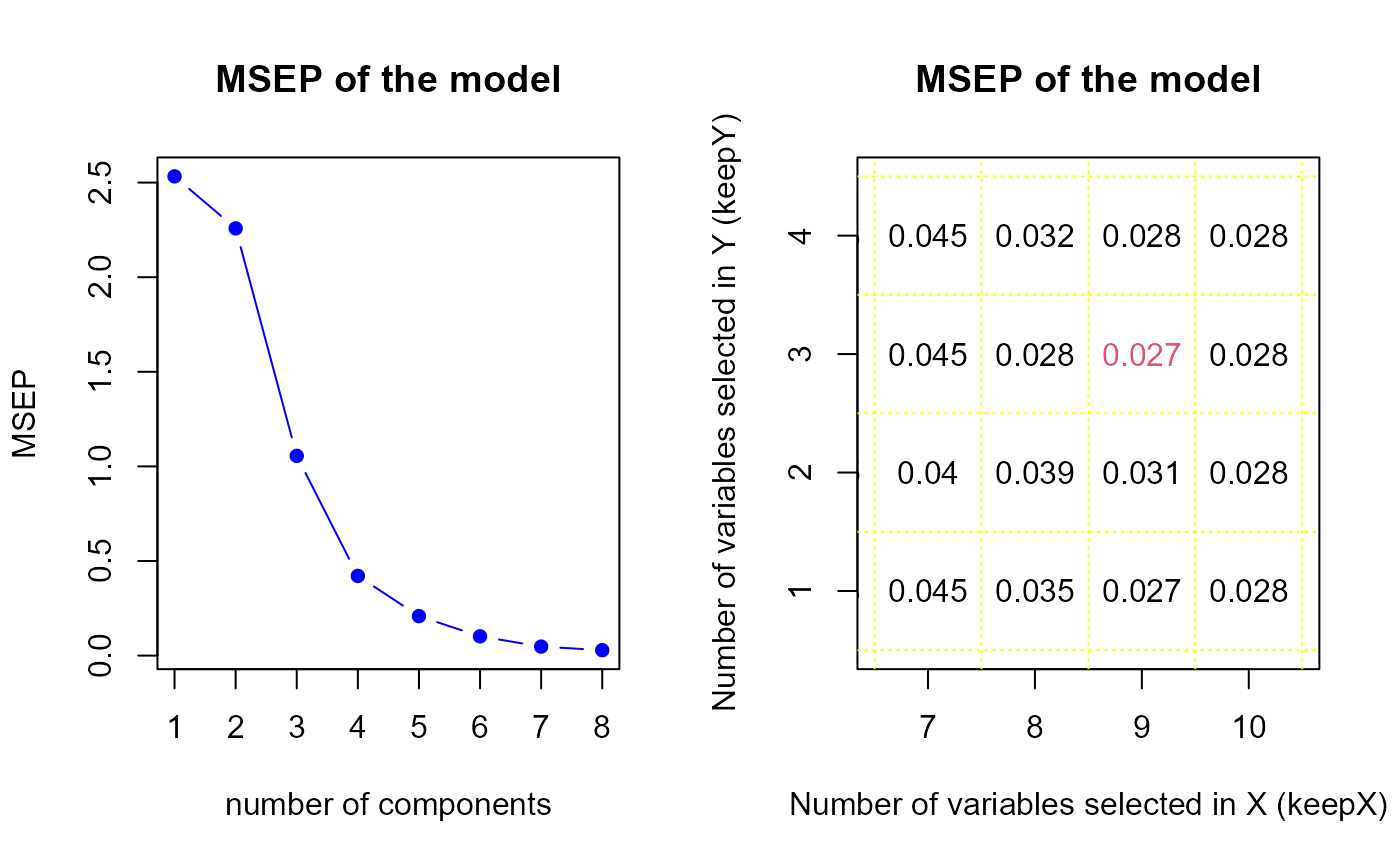

h.best <- perf.res2$h.best
keepX.best <- perf.res2$keepX.best
keepY.best <- perf.res2$keepY.best

The perf.sPLS gives us a optimal components number equal to $H =$ 8, therefore we suggest to select 8 components in our first model. It indicates us also to select 9 variables in $X$ and 3 variables in $Y$.